random readings

transformer & multi-head attention

A general explanation: {Ref-Medium}
A code implementation: {Ref}

The essence of multi-head attention is let the model calculate the weight of each value according to the position (context), this is done the formula:

   

Where

Q

is

Query

,

K

is

Key

,

V

is

Value

,

d_k

is the dimension of the network.

Q

and

K

are the positional.

This medium post gives a graphic illustration of the process: {Link}

This blog has a series of posts explain the natural language processing. I found it is very detailed with many figures explaining how weights of each layers distribute. {Link}

Embedding layers

Ref: {Link}
It is a map reduce the dimension of the input samples. For instance, sequences from combination of 50 words (n_vocabulary=50) will be reduced to 8 values after embedding.
It usually follows the One-Hot.

regress probability distribution

Simply return the mean and standard deviation, it seems comparing 2 loss functions.
{Medium-Link}
Author mentioned Kaiming initialization help training converging.
{Medium-Kaiming initinization}
The kaiming initialization consider the non-linearity of activation functions, such ReLU:

   

The post is math heavy, which can be beneficial. Read it for relaxation.

Recurrent Neural Network and LSTM

Ref: {wikipedia-LSTM}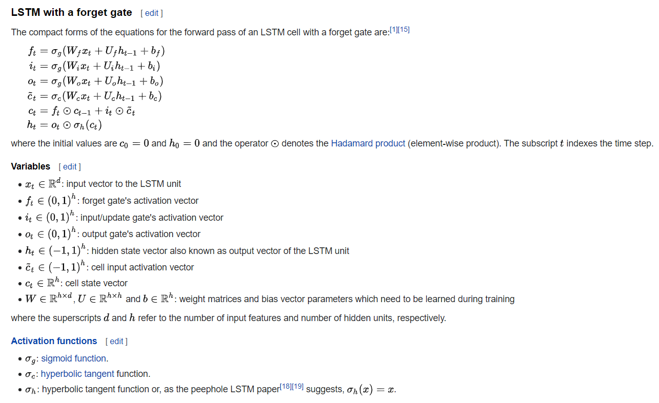


To anticipate a stochastic pattern (e.g., Markov Chain), the output/prediction from previous state flows back to adjust the probability of next prediction by leverage the impact from inputs (input gate’s activation vector), historical tendency assessment (forget/long-short-term), and output (output gate’s activation vector).

Milestone papers reading

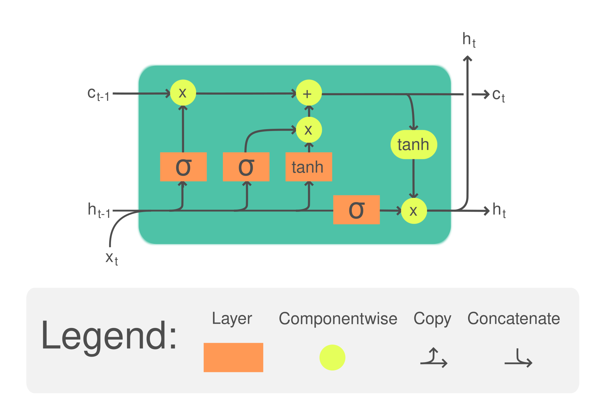
BYOL

Bootstrap Your Own Latent {ArXix}
The result of this paper is a bit dodgy. They even has disclaimer on reproducibility issue (see Border Impact Section). But the idea may be inspiring.

Highlight:

1. Didn’t use negative pair, as most Adversarial frameworks do.
   PS: Most adversarial framework boost differentiation ability of the model by joint objective that maximize similarity between postive pairs and minizie confusion between negative pairs. Mathmatically,

      

   , where is the model for positive pair, and is the model for negative pair.
2. Strictly, only online model is updated, target (offline) model passively updates as the exponential moving average of online model, in math
   , where decay rate
   Indicated in figure below by purple arrow .
3. They claim this is a Unsupvised learning method. They only keep the encoder as the final outcome.
4. Many experiments includes, a long Appendix (A-J) verifying different hypotheses.

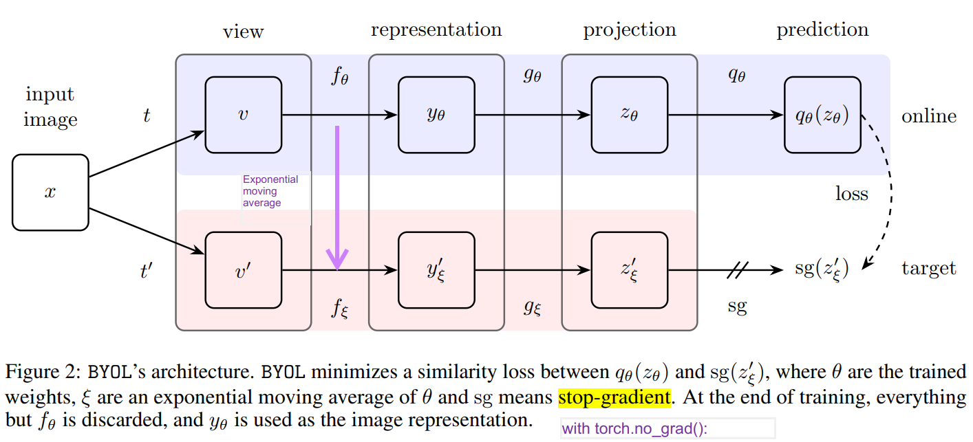
Generative Pre-trained from Pixel

The conference page{Link}
Another paper with more illustrative schematic plot {Link}
1121 understanding:
Highlight:

1. unsupervised pre-train with resized and sequentialized photos
   (Resize to save compu-resouces. sequen to fit the transformer manner)
2. linear probe show middle latent layer has most contribution
3. supervised with few labelled dataset reached 99% accuracy on CIFAR-10
   (They claim joint loss function, , is more effective.)

Framework

I-GPT (Image GPT) first pretrain with raster-scan sequentializatized photo, such as AutoRegression (some halved show below) or BERT (randomly knock off pixels to ignore influence from adjacent pixel)

NIN – Network in Network (Lin et al., 2014)

This is used in EQtransformer, so I read this paper.
The NIN idea enable nonlinear kernel operations and Global Average Pooling (compress each feature map in certain depth into 1 scalar) because each final feature map is more robust now.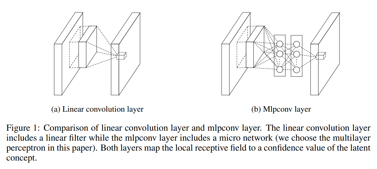

Deep residual Learning for Image Recognition

{Link}
The paper uses a hypothesis-verification architecture to prove the residual connection (convolution layer with 1*1 kernel size) mitigate the underfitting for very deep network, such as VGG (with 18 convolution layers).

Another highlight of the paper is the Implementation section, where they reveals their training scheme as well as detailed hyperparameter settings. That can be a very good guide for freshmen like me.

GoogleNet: Inception

Ref: google GoogLeNet, 2014
1*1 convolutions with fewer output channels than input channels reduce filter dimensionality and return feature cubes with smaller depth. (Consider a Primary Component Analysis)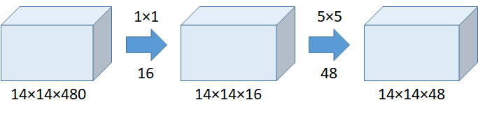

Besides, Global average pooling significant cut down the computational resources by only passing mean value of each feature map to fully connected layer compared to the feature map flattening in AlexNet. This is less prone to overfitting despite of 0.6% loss on accuracy.

Embed Physics in deepL | handle sample scarcity

Tunning papers

Channel pruning

Learning Efficient Convolutional Networks through Network Slimming, 2017 {arXiv}

They prove the efficacy with VGG net by reducing model size from 155MB to 8MB.
Users can assign a conservatively large channel size for all layers and remove those channels with the channel scaling factor below a user-defined threshold value.

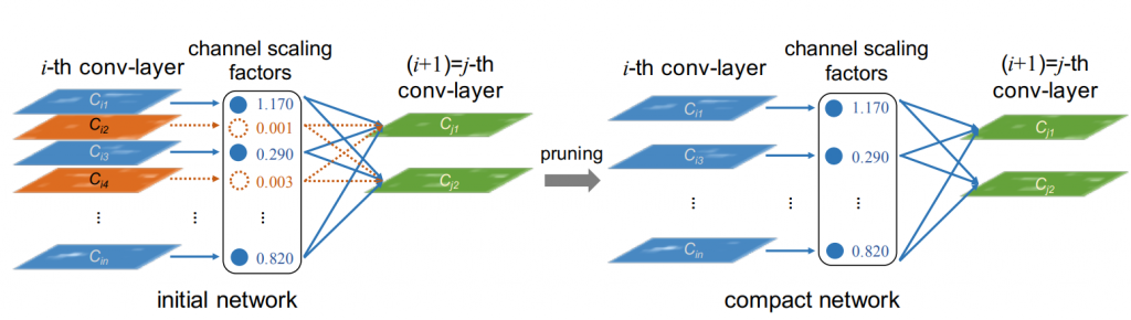
Albeit innovative, these pruning should involve only after satisfying performance reached on the preliminary model with redundancy. The paper approach 77.1% with all 512 channels layers but the test accuracy grows up a bit to 80% after pruning.

LSTM

1st Systematic Deep learning tuning instruction

The novel instruction is released in 2023, {github}. It systematically compiles methodology and implementation of hyperparameters tunning / searching in field of deep learning.

A quick skim over it help me confirm my intuitions on model design and hyperparameters searching that start from reproducing and transfer leanring set up baseline and progressively explore improvements. Their comparision on scheduler, optimizer, and exploration/exploitation trade-off are valuable for future research. They prefer random search to black-box optimization.

styleGAN-Renaissance of signal processing in Deep Learning

• Github {Link}
• Lambda lab {Link}

My brief summary:
Improve texture affine with customized window-filters in fourier domain.
Share similar philosophy with FNO, that linear manipulation in fourier domain equals multiplication in time domain (photo domain in graphic case).
Bridging downsampling and upsampling, i.e, discrete Z(x) and continous z(x) signal conversion, with sampling function and dirac impulse function.

Highlight:
Allow quick implementation of transfer learning with custom dataset. {github-Link}

Multimodal deep learning

A new ArXiv paper summarized the advances in this realm. https://arxiv.org/abs/2301.04856
The multimodal here implies data in different mode, e.g., caption generation for text, picture generation from text, etc.

Semantic Segamentation 语义分割

CSDN的解释：{Link}
初步理解为图像中的前景和后景识别，常通过卷积神经网络训练实现。
下文附源码，链接：{Link}

#--------------------------
# USER-SPECIFIED DATA
#--------------------------

# Tune these parameters

num_classes = 2
image_shape = (160, 576)
EPOCHS = 40
BATCH_SIZE = 16
DROPOUT = 0.75

# Specify these directory paths

data_dir = './data'
runs_dir = './runs'
training_dir ='./data/data_road/training'
vgg_path = './data/vgg'

#--------------------------
# PLACEHOLDER TENSORS
#--------------------------

correct_label = tf.placeholder(tf.float32, [None, IMAGE_SHAPE[0], IMAGE_SHAPE[1], NUMBER_OF_CLASSES])
learning_rate = tf.placeholder(tf.float32)
keep_prob = tf.placeholder(tf.float32)

#--------------------------
# FUNCTIONS
#--------------------------

def load_vgg(sess, vgg_path):

  # load the model and weights
  model = tf.saved_model.loader.load(sess, ['vgg16'], vgg_path)

  # Get Tensors to be returned from graph
  graph = tf.get_default_graph()
  image_input = graph.get_tensor_by_name('image_input:0')
  keep_prob = graph.get_tensor_by_name('keep_prob:0')
  layer3 = graph.get_tensor_by_name('layer3_out:0')
  layer4 = graph.get_tensor_by_name('layer4_out:0')
  layer7 = graph.get_tensor_by_name('layer7_out:0')

  return image_input, keep_prob, layer3, layer4, layer7

def layers(vgg_layer3_out, vgg_layer4_out, vgg_layer7_out, num_classes):

    # Use a shorter variable name for simplicity
    layer3, layer4, layer7 = vgg_layer3_out, vgg_layer4_out, vgg_layer7_out

    # Apply 1x1 convolution in place of fully connected layer
    fcn8 = tf.layers.conv2d(layer7, filters=num_classes, kernel_size=1, name=fcn8)

    # Upsample fcn8 with size depth=(4096?) to match size of layer 4 so that we can add skip connection with 4th layer
    fcn9 = tf.layers.conv2d_transpose(fcn8, filters=layer4.get_shape().as_list()[-1],
    kernel_size=4, strides=(2, 2), padding='SAME', name=fcn9)

    # Add a skip connection between current final layer fcn8 and 4th layer
    fcn9_skip_connected = tf.add(fcn9, layer4, name=fcn9_plus_vgg_layer4)

    # Upsample again
    fcn10 = tf.layers.conv2d_transpose(fcn9_skip_connected, filters=layer3.get_shape().as_list()[-1],
    kernel_size=4, strides=(2, 2), padding='SAME', name=fcn10_conv2d)

    # Add skip connection
    fcn10_skip_connected = tf.add(fcn10, layer3, name=fcn10_plus_vgg_layer3)

    # Upsample again
    fcn11 = tf.layers.conv2d_transpose(fcn10_skip_connected, filters=num_classes,
    kernel_size=16, strides=(8, 8), padding='SAME', name=fcn11)

    return fcn11

def optimize(nn_last_layer, correct_label, learning_rate, num_classes):

  # Reshape 4D tensors to 2D, each row represents a pixel, each column a class
  logits = tf.reshape(nn_last_layer, (-1, num_classes), name=fcn_logits)
  correct_label_reshaped = tf.reshape(correct_label, (-1, num_classes))

  # Calculate distance from actual labels using cross entropy
  cross_entropy = tf.nn.softmax_cross_entropy_with_logits(logits=logits, labels=correct_label_reshaped[:])
  # Take mean for total loss
  loss_op = tf.reduce_mean(cross_entropy, name=fcn_loss)

  # The model implements this operation to find the weights/parameters that would yield correct pixel labels
  train_op = tf.train.AdamOptimizer(learning_rate=learning_rate).minimize(loss_op, name=fcn_train_op)

  return logits, train_op, loss_op

def train_nn(sess, epochs, batch_size, get_batches_fn, train_op,
             cross_entropy_loss, input_image,
             correct_label, keep_prob, learning_rate):

  keep_prob_value = 0.5
  learning_rate_value = 0.001
  for epoch in range(epochs):
      # Create function to get batches
      total_loss = 0
      for X_batch, gt_batch in get_batches_fn(batch_size):

          loss, _ = sess.run([cross_entropy_loss, train_op],
          feed_dict={input_image: X_batch, correct_label: gt_batch,
          keep_prob: keep_prob_value, learning_rate:learning_rate_value})

          total_loss += loss;

      print(EPOCH {} ....format(epoch + 1))
      print(Loss = {:.3f}.format(total_loss))
      print()

def run():

  # Download pretrained vgg model
  helper.maybe_download_pretrained_vgg(data_dir)

  # A function to get batches
  get_batches_fn = helper.gen_batch_function(training_dir, image_shape)

  with tf.Session() as session:

    # Returns the three layers, keep probability and input layer from the vgg architecture
    image_input, keep_prob, layer3, layer4, layer7 = load_vgg(session, vgg_path)

    # The resulting network architecture from adding a decoder on top of the given vgg model
    model_output = layers(layer3, layer4, layer7, num_classes)

    # Returns the output logits, training operation and cost operation to be used
    # - logits: each row represents a pixel, each column a class
    # - train_op: function used to get the right parameters to the model to correctly label the pixels
    # - cross_entropy_loss: function outputting the cost which we are minimizing, lower cost should yield higher accuracy
    logits, train_op, cross_entropy_loss = optimize(model_output, correct_label, learning_rate, num_classes)

    # Initialize all variables
    session.run(tf.global_variables_initializer())
    session.run(tf.local_variables_initializer())

    print(Model build successful, starting training)

    # Train the neural network
    train_nn(session, EPOCHS, BATCH_SIZE, get_batches_fn, 
             train_op, cross_entropy_loss, image_input,
             correct_label, keep_prob, learning_rate)

    # Run the model with the test images and save each painted output image (roads painted green)
    helper.save_inference_samples(runs_dir, data_dir, session, image_shape, logits, keep_prob, image_input)

    print(All done!)

#--------------------------
# MAIN
#--------------------------
if __name__ == '__main__':
    run()