[Math for Fun] Statistics in ML
ML skills
Different clustering with Toy dataset
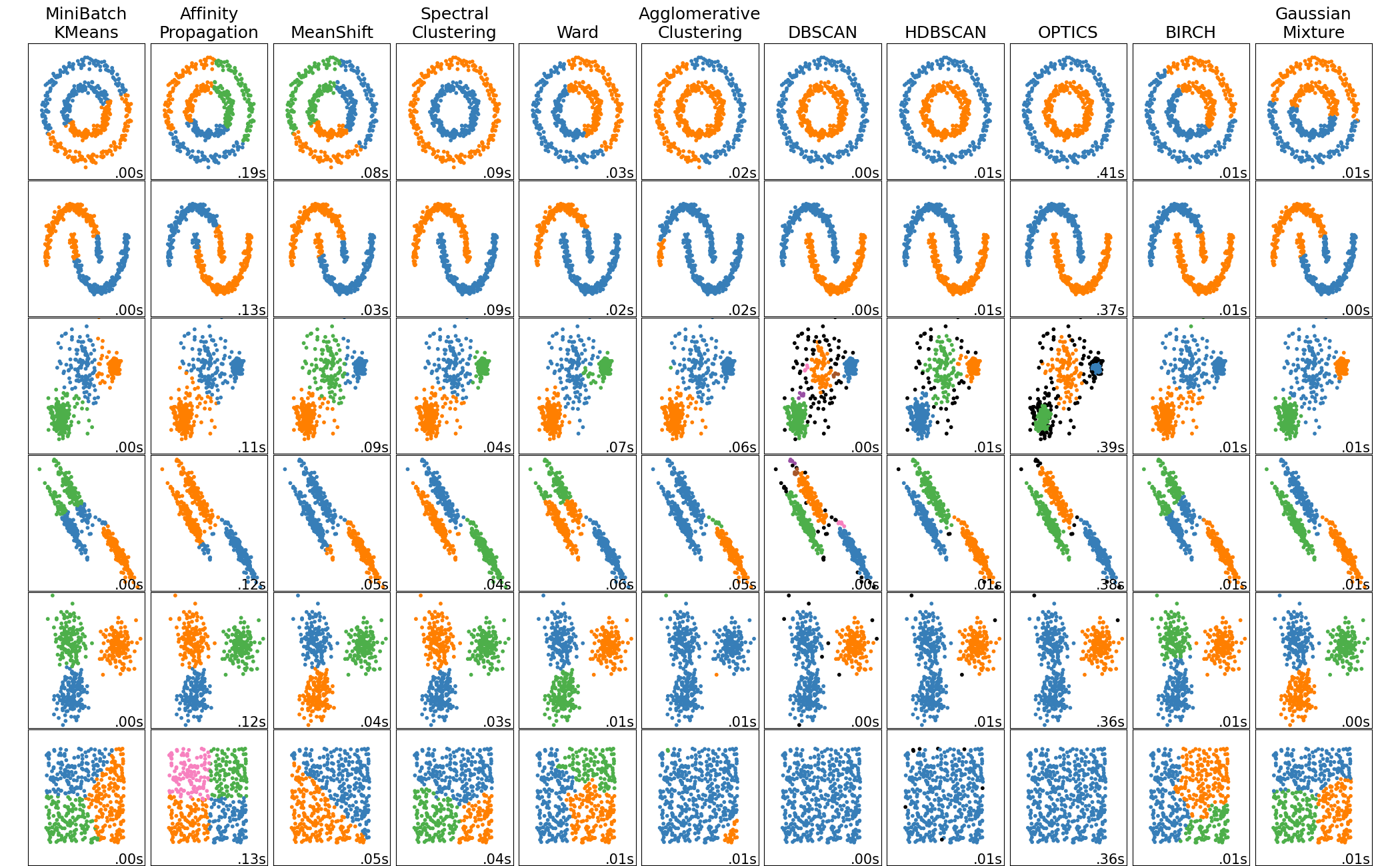
Found this post from sklearn with intuitive illustration of different clustering approaches.
Can play with the math behind.
{Ref}
PINN
Physical information neural network
A 1-D example is axial displacement of a column under axial load in given pattern.
The strain can be expressed as a partial derivative equation:
A PDE need to be solve:
|
1 |
\frac{\mathrm{d}^2u}{dx^2}=\frac{-2(a+a^3b(b-x+1))}{{(a^2b^2+1)}^2} |
and boundary condition:
|
1 2 |
u(0)=u(1)=0\\ a=50, x_b=0.8,b=x-x_b |
- Independent variables: x(input)
- Dependent variables: u (outputs)
Derive u(x) for all x in range [0,1]
The exact solution is given by
|
1 |
u(x)=(1-x)(arctan(ab)+arctan(ax_b)) |
Our f is $$f = \frac{\mathrm{d}^2u}{dx^2}+\frac{2(a+a^3b(b-x+1))}{{(a^2b^2+1)}^2}$$
The neural network is regression of the equation as well as the target.
Advantages:
- less data
- good for complex math equation
- no need to solve the pde
Drawback:
- large iterations
XGBoost
是一种基于树模型提出的并行式计算方法
发展:
|
1 2 3 4 5 |
graph TD; DecisionTree -->Bootstrap; Bootstrap --> GradBoostDecisionTree; RandomForest-->GradBoostDecisionTree; GradBoostDecisionTree-->XGBoost; |
其前身是GBDT – Gradient Boosting Decision Tree
-
CSDN 对于GBDT的解释:
https://blog.csdn.net/yyy430/article/details/85108797 -
CSDN-XGBoost理论:
https://blog.csdn.net/v_JULY_v/article/details/81410574 -
手写推导与代码实现:
https://zhuanlan.zhihu.com/p/143009353
具体实现可以采用python的xgboost库
其主要改进是剪枝算法的软硬件加速
老赵说目前主流的方法是这些,需要注意学习。
PCA(Primay Component Analysis)
by StatQuest
For a 4D example:
- Decentralized: count the mean point, and move the central point of entire sample group to the original point.
- Solve Eigenvectors: direction with minimum variation (Sum of Square Distance–SS(distance))
- SSD = Eignvalue for PC1
- sqrt(Eignvalue for PC1) = Singular Value for PC1
- SVD(Singular value decomposition): Rotate the Eigenvalue to primary axis
- Dimension Reduction/Screen Plot: If PC1 and PC2
- Compute variation of PC1 = SS(distance for PC1)/(n-1)
- Trivial PC can be ignored.
Stats & Maths
t-test
especially independent t-test
{Wiki-ref}
{scipy-ref}
{t-test explanation}
Distribution.log_prob() & nn.GaussianNLLLoss
Negative Log
Because logarithm’s simplicity and efficiency in converting multiplication into summation,
|
1 |
f(x)=\frac{1}{\sigma\sqrt{2\pi}}e^{-\frac{1}{2}(\frac{x-\mu}{\sigma})^2} |
By negative log
|
1 |
-log[f(x)]=\frac{1}{2}(\frac{x-\mu}{\sigma})^2+log(\sigma)+log(\sqrt{2\pi}) |
Back to difference of the 2 implementation
parameter definition difference
All summary are drawn from official doc {GNLLss} {Distribution.log_prob}
First in log_prob, self.loc is mean, self.scale is standard deviation (stddev):
|
1 |
stddev = \sqrt{\frac{\sum(x-\mu)^2}{N}} |
But in GNLLLoss, input parameters are input, target, var, where input is mean value \mu, var is variance s^2, target is the observation. Both input and var are generated by the network.
|
1 |
Variance = s^2 = \frac{\sum(x-\bar{x})^2}{n-1} |
You may notice, stddev has denominator N while Variance has that as n-1. My view is that stddev is a probability parameter, hence, N is the total sample counted in the probability distribution, however, Variance is statistic parameter, so n is the number of observations, n-1 reflect the \sum{(x-\bar{x})^2} operation in nominator has 1 less degree of freedom than \sum{x^2}.
Other interesting strategy optimizing the computation efficiency comprises that:
- Neglecting the constant value
log{(\sqrt{2\pi})} - reduction by mean instead of sum
- set a safety value of 1e-6 to avoid ZeroDividor Error
These approach can be verified by setting the GNLLLoss to:
|
1 2 3 4 5 6 |
loss = torch.nn.GaussianNLLLoss(full=True, eps=1e-4, reduction='sum') loss(dists.mean, tgt, dists.stddev**2) def nll_loss(observations, dists): return -dists.log_prob(observations).sum() nll_loss(tgt, dists) |
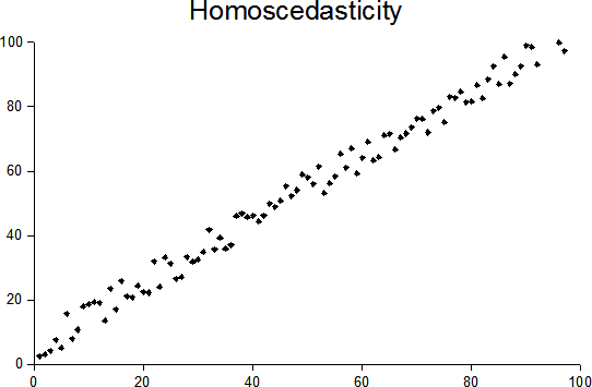
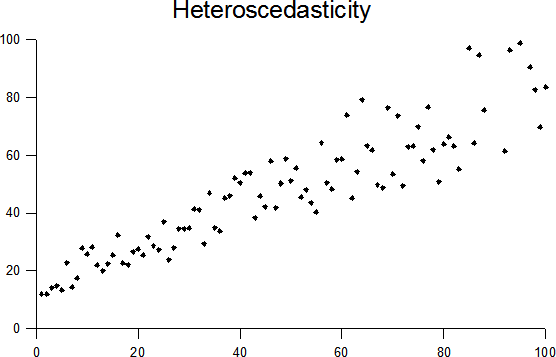
It mentioned in some case var array can have less dimension that mean due to homoscedasticity assumption, which explained below.
homoscedasticity
The takeaway is homoscedastic means regard variance the same for all samples in certain dimension. The antonym is heteroscedastic.
{Ref}
SNR
ddof: diviser of degree of freedom
|
1 |
s = \sqrt{\frac{(x-\bar{x})^2}{N-ddof}} |
In Statistic:
|
1 |
SNR = \frac{\bar{x}}{s} |
In Audio processing, decibels preferred

|
1 |
P_{signal} = E(s^2)=(A_{signal})^2 |
Central Limit Theory
No matter what distribution that samples are taken from, their mean value are in normal distribution. (Cauchy Dist seems not obey this rule.)
Its advantages is that the mean value probability is independant to the original data distribution.
R2 coefficient of correlation
Also based on sklearn. Most importantly, a validation standard is proposed, the coefficient of determination. In sklearn, it is called r2_score.
R^2=1-\frac{(\sum_{i}{(y_i-(yi ) ̂ )^2 )}}{(\sum{i}{{(y_i-\bar{y})}^2}}=1-\frac{MSE}{VAR(y)}
|
1 |
R^2 = 1-\frac{\sum_{i}{(y_i-\hat{y_i})^2}}{\sum_{i}{(y_i-\bar{y})^2}}=1-\frac{MSE(\hat{y})}{VAR{(y)}} |
An more comprehensive explanation is
|
1 2 3 4 5 |
\hat{y} = \frac{1}{n}\sum_{i=1}^{n}{y_i}\\ SSR = SS_{reg}=\sum{(\hat{y_i}-\bar{y})^2}\\ MSE = SSE = SS_{res}=\sum{({y_i}-\hat{y})^2}\\ VAR(y_i) = SST = SS_{total} = \sum{({y_i}-\bar{y_i})^2} = SSR+SSE \\ SSR/SST = \frac{SST-SSE}{SST} = 1-\frac{SSE}{SST} = 1-\frac{MSE}{VAR{y_i}} |
You may wonder why SST = SSR + SSE
|
1 |
\sum{(y_i-\bar{y})^2}=\sum{[(y_i-\hat{y})+(\hat{y_i}-\bar{y})]^2} = \sum{[(y_i-\hat{y})+(\hat{y_i}-\bar{y})]^2} |
For more information, please refer to the link below:
https://blog.csdn.net/u012841922/article/details/78691825
Origin of exp (Euler’s constant)
源自最大利率问题中发现
Originated from maximal interest problem in investment
|
1 |
lim_{n \rightarrow \infty}{(1+1/n)^{n}}=e |
Then in case that basic interest rate is 1/n. We simply multiply MARKDOWN_HASH878bd532f1718635c637124be801e4d9MARKDOWNHASH by x.
$$
lim{n \rightarrow \infty}{(1+x/n)^n}=lim_{n \rightarrow \infty}{[(1+x/n)^{n/x}]^x}=e^{x}=exp(x)
$$
Proof of unbiased estimation of STDV
Why there is n-1 in denominator of the estimation of STDV (Standard Deviation)
The inituitively correct STDV is biased deviation for it does not consider the error between average of each sampling and the real mean value of the entire distribution.
Let us set
TSS (Total Sum Square-error)
RSS (Real Sum Square-error)
ESS (Error Sum Square-error)
|
1 2 3 |
TSS = \sum^n_{i=1}{(x_i-\mu)^2} \\\\ RSS = \sum^n_{i=1}{(x-\bar{x})^2} \\\\ ESS = \sum^n_{i=1}{(\bar{x}-\mu)^2} \\\\ |
It can easily prove that:
|
1 2 3 4 5 |
TSS = \sum^n_{i=1}{[(x_i-\bar{x})-(\bar{x}-\mu)]^2}\\\\ =\sum^n_{i=1}{(x-\bar{x})^2}+\sum^n_{i=1}{(\bar{x}-\mu)^2}-2\sum^n_{i=1}{(x-\bar{x})(\bar{x}-\mu)}\\\\ =\sum^n_{i=1}{(x-\bar{x})^2}+\sum^n_{i=1}{(\bar{x}-\mu)^2}\\\\ =RSS+ESS |
At the same time,
|
1 2 |
ESS = \sum^n_{i=1}{(\bar{x}-\mu)^2} = \sum^n_{i=1}{[\sum^n_{i=1}{(\frac{x_i}{n}})-\mu]^2}\\\\ |
Take out the denominator n, we got
|
1 2 3 |
=\frac{1}{n^{2}}\sum^n_{i=1}{[ \sum^n_{i=1}{(x_i)}-n\mu]^2} \\ = \frac{1}{n^{2}}\sum^n_{i=1}{[ (x_1-\mu) + (x_2 - \mu)+...+(x_n-\mu)]^2}\\ = \frac{1}{n^{2}}\sum^n_{i=1} \sum^n_{i=1}{[(x_i-\mu)^2 + \sum_{i\ne j}{(x_i-\mu)(x_j-\mu)]}} |
It assume the x_i is a random distribution, so the multiplication of all i \ne j samples are negligible high-order minors.
|
1 2 3 4 |
\approx \frac{1}{n^{2}}\sum^n_{i=1} \sum^n_{i=1}{[(x_i-\mu)^2]} \\ = \frac{1}{n^{2}} n \sum^n_{i=1} {[(x_i-\mu)^2]}\\ = \frac{1}{n} \sum^n_{i=1} {[(x_i-\mu)^2]} = \frac{1}{n} TSS |
To wrap up:
|
1 2 3 4 |
\because ESS \approx \frac{1}{n} TSS \land TSS = RSS + ESS\\ \therefore RSS = TSS - ESS \approx (1-1/n)TSS = \frac{n-1}{n}TSS \\ \therefore \frac{RSS}{n-1} \approx \frac{TSS}{n} \\ \therefore \frac{\sum^n_{i=1}{(x_i-\mu)^2}}{n} \approx \frac{\sum^n_{i=1}{(x-\bar{x})^2}}{n-1} |
Thus, unbiased estimation using n-1 as denominators is preferred when sample size is small (say\<30), or highly possible to be biased from true distribution.
Ref:
- Math deduction:
http://www.360doc.com/content/18/0924/22/48898194_789378974.shtml - Code validation:
https://stats.stackexchange.com/questions/249688/why-are-we-using-a-biased-and-misleading-standard-deviation-formula-for-sigma
This might be the start of Complex Functions.
Great thanks to 3Blue1Brown\’s video for the inspiration.
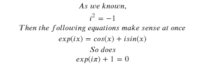
When it comes to exp([imaginery numbers]),
it is more appropriate to consider exp as a polynomial function with infinite factorial terms as shown below instead of taking it as multiple productions of the operand itself in the situation exp([real number]).
This is defined by Taylor\’s series expansion.
In my view, these series equations only valid at x=0.
However, we won\’t put too much attention on it here.
For further info, you may go to this link in Zhihu.
exp to Euler\’s formula
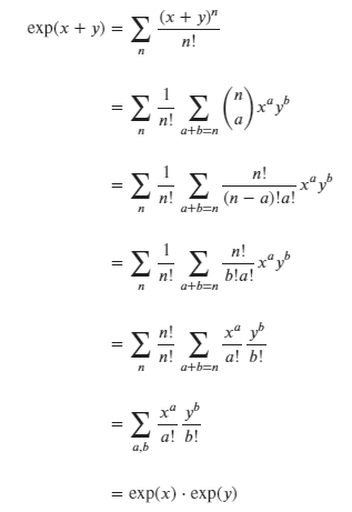
 ### The proof of exp(a)*exp(b) = exp(a+b)
This is the homework for the video of 3Blue1Brown.
QR factorization
|
1 2 |
A = QR\\\\ Q^T A = Q^T Q R = R |
A is a random matrx, R is upper triangular matrix, Q is a orthogonal matrix usually built by Gram-schmit method (find a set of orthogonal vectors from any 3 linear independent vectors)
This method takes advantage of orthogonality of Q matrix to numerically solve the upper triangular matrix of A. The R takes less storage space and easier to find inverse.
Gaussian Process with Bayes rule
$$ P(w|y, x) = \frac{p(y, x, w)}{p(y, x)} = \frac{p(y|x,w)p(x)p(w)}{p(y|x)p(x)}=\frac{p(y|x,w)p(w)}{p(y|x)}$$
Stats and ML
Logistic Function
Consider a random animal species on a island, the population W is function of time t, which is W(t).
For a short term, With abundant resources, the birth rate is a constant \alpha. Mathematically, \frac{dW(t)}{dt} = \beta W(t)
For a long term, the birth rate will gradually drop to zero. Mathematically,
\frac{dW(t)}{dt} = (\beta - \phi) W(t)
As the amount of drop \phi will be a function of population, too. There is
\frac{dW(t)}{dt} = (\omega - W(t)) \widetilde{\beta} W(t)
Notice that now: \omega\widetilde{\beta} where \omega has the meaning of maximal population.
Now a trick on math is define a normalized ratio P(t)=W(t)/\omega
And \frac{dP(t)}{dt} = \frac{1}{\omega} \frac{dW(t)}{dt} = \frac{1}{\omega} (\omega - W(t)) \widetilde{\beta} W(t) = \omega\widetilde{\beta} P(t)(1-P(t))
Tide it up to \frac{1}{P(t)(1-P(t))} dP(t) = \beta dt, and integrate both sides.
log{\frac{P(t)}{1-P(t)}} = \beta t + \alpha
P(t) = \frac{exp(\alpha + \beta t)}{1+exp(\alpha + \beta t)}
Get normal distribution from max entropy assumption
To be more mathematical, we paraphrase the task as below.
\widehat{p(x)} = \underset{s.t. \int{p(x)dx}=1, \int{xp(x)dx}=\mu, \int{(x-\mu)^{2}p(x)dx}=\sigma^{2}}{max{[-\int{p(x)log{p(x)}dx}]}}
The following part is not completed, but I am too annoyed since the original file is lost without auto-save
Lagrange multiplier:
Partial derivation \frac{\partial{L}}{\partial{p(x)}}
The p(x) is even, so \lambda_2=0
Let e^{\lambda_1 - 1} = c, and \lambda = -\lambda_3
By polar coordinate integration, \int{e^{-\frac{\pi}{2}}dx}=\sqrt{2\pi}
The \lambda=\frac{1}{2\sigma^2}
Therefore, p(x)=\frac{1}{\sqrt{2\pi}\sigma}e^{-\frac{(x-\mu)^2}{2\sigma^2}}
Precision Recall F-score
Ref: {Link}
For a confusion matrix
| Actual/Pred | Negative | Positive |
|---|---|---|
| Negative | True Negative | False Positive |
| Positive | False Negative | True Positive |
The ‘True’ and ‘False’ are comment for prediction.
|
1 2 3 4 5 |
Precision = \frac{TP}{TP+FP} = \frac{TP}{(All-pred-P)}\\ \\ Recall = \frac{TP}{TP+FN} = \frac{TP}{(All-actual-P)}\\ \\ fscore = 2*\frac{Prec*Reca}{Prec+Reca} = {(\frac{1}{Prec}+\frac{1}{Reca})}^{-1} |
fscore is useful when seeking balance between precision and recall, or with unbalanced dataset.
kernel function in SVM
Support vector machine
Kernel functions are applied on the input data, somewhat like the convolution layers, for feature extraction
Kernel functions are implicit form of mapping function.
In application, we define kernel function but not mapping function, because the calculation of kernel function is simpler than mapping function.
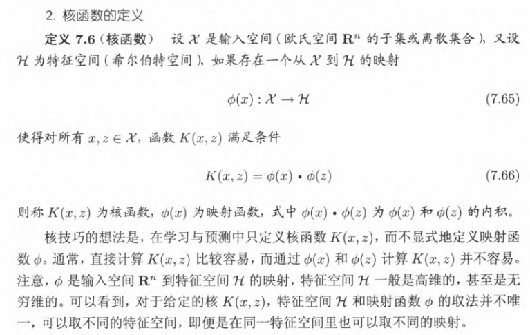
Ref: 《统计学习方法》- by 李航, from 清华大学
Also with a example of ellipse that may help
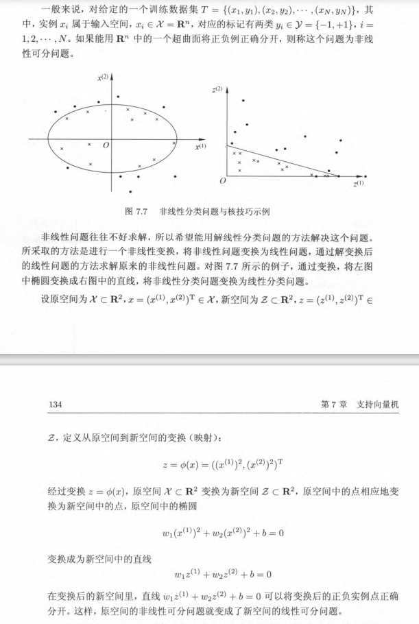
I personally conclude that kernel function mapping the inner product of input vector to a space with higher dimension, wrapping the input up like a kernel, so that the low-dimensional (usually 1-D) parameters (w & b) can be optimized in a non-linear case as that in the linear case.