Coding Guides

systematic tutorial

The tutorial describe a integral workflow of transfer learning {Link}, experiment tracking, and finally model deploy.

It is a perfect example to follow with detailed source code and notebook for each chapter.

However, to boost the productivity, using new libraries like

pytorch-lightning

,

ignite

(integration, like

kera

s for

tensorflow

),

wandb

and

tensorboard

(training monitoring and hyperparameter tuning.)

Related web page:

1. {PyTorch-lightning v.s. Ignite}
   Start from PT-lightning which has quicker learning curve and better support in distributed learning.
2. {PyTorchLightning-offiical Transfer leanring doc}
   Also have other cutting edge examples, such as meta-learning and DQN for RL.

plot model architecture with tensorboard

Install tensorboard, go to bash:

conda install tensorboard
# or
pip3 install tensorboard
python operation:
import torch.utils.tensorboard as tsb

Go back to bash run tensorboard, but make sure the port is available for it.
tensorboard --logdir=%YOUR_DIR --port=%YOUR_PORT

Otherwise, just try google colab’s tutorial to load tensorboard

{Colab_Tensorboard}

{PyTorch_Tensorboard}
A imitation of Keras:
from torchsummary import summary
summary(%YOUR_NET,input_size=%YOUR_INPUT_SIZE)
# batch size not considered and denoted as -1 in return
check cuda availability
# check current GPU(s)
def device_info():
    from sys import modules
    assert "torch" in modules
    n = torch.cuda.device_count()

    print("num"+"\t"+"|device name\t\n")
    for i, device in enumerate([torch.cuda.get_device_name(i) for i in range(n)]):
        print(i, "\t", device)
#     return [torch.cuda.get_device_name(i) for i in range(n)]

device_info()
Output:
num |device name    

0    NVIDIA GeForce RTX 2080 Ti
When allocating the cuda device, we can use
device = torch.device("cuda:0")
super()
usually seen in init function

will
torch.autograd
The original code uses 
torch.Autograd


, but seems updated version uses 

torch.autograd


This zhihu post show some common application of Variable:

@ require_grad & volatile: exclude gradient, save computation resource

@ register_hook: attach a additional function to the Variable

@ profiler: Analyze the autograd and resource usage for Variables
release storage
CSDN: https://blog.csdn.net/jiangjiang_jian/article/details/79140742

@ gabarge collector: gc
import gc
print(gc.get_threshold()) # check renew threshold
gc.collect()  # manual release storage
apex
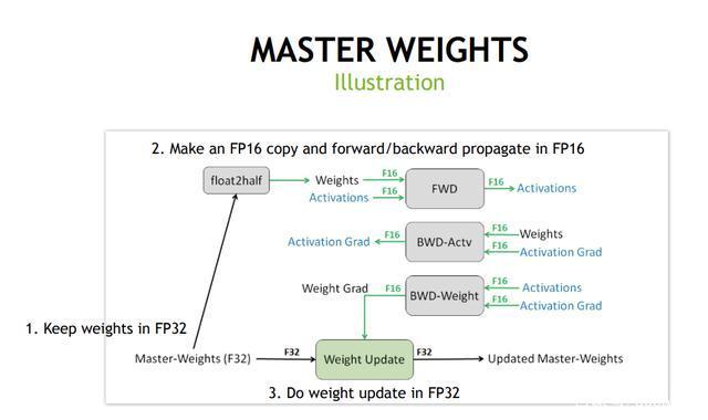
apex.amp {知乎介绍}
其中 amp: Automatic Mixed Precision

混合精度训“在内存中用FP16做储存和乘法加速计算，用FP32做累加避免舍入误差”。
opt_level = 'O1' 根据黑白名单自动选择储存精度

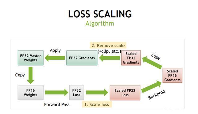
Dynamic Loss Scalling动态损失放大，以适应FP16较窄的值域
{Nvidia官方文档}
amp.scale_loss
It should consist of automatically scaling FP32 Weights to FP16 and scaling FP16 grad to FP32.

Explanation from 【Official Doc of Apex】
with amp.scale_loss(loss, optimizer) as scaled_loss:
    scaled_loss.backward()
Usually use it with Context Manager**
graphs explanations


Graphs from Baidu
mseed
A format from SEED (Standard for the Exchange of Earthquake Data)

Can be easily operated by matlab

【Read miniSeed Files-CNblogs】
obspy
opensource package for earthquake research

【CSDN】
HDF5
Hiearchical Data Format version 5

This is built for fast data operation in python numpy

A HDF file mainly has groups and datasets.

Like file folders and arrays.

It can also set metadata (e.g., attributes)

【Official Doc】

There is also an book by O'Relly

{Quick Start-CSDN}
When load data with 
f['X']
, you only load a generator, you can modify the data directly, but you can't read the dataset once you close the file. For instance:

If you solely want a copy of the dataset in hdf5:
with h5py.File("mytest.hdf5", "r") as f:
    dtset_load = f['X'][:]
dtset_load.shape
You will get error: 
Not a dataset (not a dataset)
 if you do this:
with h5py.File("mytest.hdf5", "r") as f:
    dtset_load = f['X']
dtset_load.shape
Because the file has been closed outside 
with
, the generator expired, too.
argparse
A Chinese introduction on 【Zhihu】

Here is part of the example:

@ ap.ArgumentParser(): A loader object

@ parser.add_argument()

@@'--%var_name%'

@@required: bool type, is this var compulsory

@@default：initial value for this var
import argparse as ap

parser = ap.ArgumentParser(description='姓名')
parser.add_argument('--family', type=str, help='姓')
parser.add_argument('--name', type=str, required=True, default='', help='名')
args = parser.parse_args()

#打印姓名
print(args.family+args.name)
Colab
definitely worth trying.

【20 productive Tricks for Colab】

Useful commands are:

@!bash

@tensorboard

@interactive tables for dataframe
but note that it will frequently re-mount google cloud disk.

【tips for long-term training with Colab】
Function Understanding
BCEWithLogitsLoss
BCE is binary cross entropy and with Logit just add a Sigmoid at the input 
X_n
 for numeric stability in training.
{This TowardDatascien Post} explains the math in BCELoss.

It says the CELoss is the KL divergence between the Cross Entropy and Entropy, namely:
$$ D{KL}(q||p)=H{p}(q)-H(q)=\sum{c=1}^{C}q(y{c})\cdot[log(q(y_c))-log(p(y_c))] $$
Where 
H_{p}(q)
 is cross entropy, 
H(q)
 is entropy, 
p(x)
 is the hypothetical prob dist, 
q(x)
 is the target prob dist.

The cross entropy in a binary scenario turns into the formulas below.
$$ BCELoss = 1/n\sum(y_n \cdot \ln{x_n} + (1-y_n) \cdot \ln{(1-x_n)}) $$
To make 
x_n
 varies from 0 ot 1, corresponding to target 
y_n=\lbrace0,1\rbrace
. Add an sigmoid function on prediction 
x_n
, we have
$$

BCEWithLogitsLoss = 1/n\sum(y_n \cdot \ln{[\sigma(x_n)]} + (1-y_n) \cdot \ln{[\sigma(1-x_n)]})

$$
where
\sigma(x) = \frac{1}{1+exp(x)}
 is also know as sigmoid function, also used in logistic regression model (might be the reason why it is called logits here)
CrossEntropyLoss & LogSoftmax
The default input of CEL (Cross Entropy Loss) are raw probability of each classification and the index of maximum. One input the individual probability of each clas. See {Official Doc}. Here only discuss the default setting.
The equation for default (one hot) Cross Entropy Loss is
l_n = -w_{y_n}\cdot log{\frac{exp(x_{n,y_n})}{\sum_{c=1}^{C}{exp(x_{n,c})}}}
Notice there is a 
log
, so the input should be original probability.

The function returns the mean CEL for each Minibatch by default.
One thing to mention is: The official doc says "The CEL is equivalent to combination of LogSoftmax and NLLLoss". Where NLL means negative log likelihood.
LogSoftmax(x_i) = log{\frac{exp(x_i)}{\sum_{j}{exp(x_j)}}}
NLLLoss(x_i) = -w_n\cdot x_i
According to StackOverflow , using 
LogSoftmax
 as the final layer and 
NLLLoss
 as loss function has equivalent effect as using 
Linear
 as final layer and 
CrossEntropyLoss
 as the loss function.
You can verify with following codes:
import torch

m = torch.nn.LogSoftmax(dim=1)
loss_1 = torch.nn.NLLLoss()
loss_2 = torch.nn.CrossEntropyLoss()

inp = torch.randn(3, 5)
tgt = torch.tensor([1, 0, 4])

# combined
out_cb = loss_1(m(inp), tgt)
# cross entropy
out_ce = loss_2(inp, tgt)

print(out_cb, out_ce)

# manually 
softmax = (inp.exp().T/inp.exp().sum(1)).T
logsoft = softmax.log()
nll = -torch.tensor([logsoft[i,j] for i,j in zip(range(3), list(tgt))]).mean()
print(nll)

# nll and out_cb, out_ce are all the same
# moreover the softmax(logsoftmax) = softmax(inp)
# try this
sfm = lambda x: (x.exp().T/x.exp().sum(1)).T
print(sfm(logsoft), sfm(inp))

Softmax, sigmoid; CrossEntropy, BCELoss
I have been confused about softmax, sigmoid, CE and BCE usage for long.

The take-home summary is:

use softmax and CrossEntropy better for muliti-class classification.
BCELoss and sigmoid better for binary one.

Refer to {Link}, that:
softmax([-2,34, 3,45])=[0.3%, 99.7%] # probability meaningful, but usually close to (0.1%, 99.9%)
sigmoid([-2.34, 3.45])=[8.79%, 96.9%] # no probability meaning, 
The Cross Entropy loss function in fact has built in the softmax:
l_n = -w_{y_n}\cdot log{\frac{exp(x_{n,y_n})}{\sum_{c=1}^{C}{exp(x_{n,c})}}}
The math expression in program can be expressed as
NLLoss(-torch.log(torch.softmax(prediction)))
What's more the pytorch official doc says the Cross Entropy loss is default doing mean on loss, so if want to see the overall loss for entire train set, better use
total_run_loss = run_loss * x.size()
Connection with KL-divergence
The CrossEntropy (Xentropy) is a pragmatic simplification of the KL-divergence \(KL(p,q)=\sum_i{(p_i \log {p_i} - p_i \log{q_i})}\), where the first term is constant for given target probability, except in model distillation that target distribution from the teacher model also changes. Thus Xentropy only minimize the second term \(\sum_i{(p_i \log{q_i})}\).
Build large model with ModuleList, ModuleDict, Sequential
Ref: {Toward_datasci}
Takeaway: Sequential build-in the forward sequentially for the modules. ModuleList hold modules like a list, commonly used in UNet. ModuleDict hold modules like a dict, commonly used for alternatively modules for baseline comparison.
debugginng multi-threading forks
When seeing multi-threading bug or warning reports, try set the 
num_worker
 variable in 
Dataloader
 to 0 to disable multiprocess data feeding.