Photogrammetry Reconstruction
Overview
This is motivated by DVPB project:
Multi-Scale Digital Twin Reconstruction of a Cliff System using Drone Photogrammetry
Climate change and global warming are introducing increasing uncertainties to cliff stability through coupled hydro-thermal-mechanical processes including seepage, swelling, freeze–thaw cycles, and creeping, and fracturing. The road above
This project aims to develop a multi-scale, multi-physics digital twin integrating:
- Macro-scale: satellite terrain and hydrology
- Meso-scale: drone photogrammetry and geomorphology
- Micro-scale: laboratory geological testing
The coupled physical processes include:
- Hydrology: seepage and infiltration
- Thermal: freeze–thaw and temperature effects
- Mechanical: swelling, creep, fracturing, and deformation
1. Motivation for Photogrammetric Reconstruction
Why a Digital Twin is Needed
Environmental loading continuously modifies cliff geometry through:
- Water seepage
- Freeze–thaw cycles
- Rock swelling
- Long-term creeping deformation
- Temperature variations
A high-resolution digital twin enables:
- Surface change detection
- Hydrological analysis
- FEM simulations
- Long-term monitoring
- Hazard assessment
Multi-Scale Framework
Macro-scale: Satellite Terrain and Hydrology
Satellite DTMs are the first readily available source of regional terrain information. However, the resolution is generally insufficient for steep cliff analysis.
| Dataset | Typical Resolution |
|---|---|
| SRTM | 30 m |
| ASTER GDEM | 30 m |
| Copernicus DEM | 30 m |
| ALOS AW3D30 | 30 m |
At this scale, the entire bowl-shaped cliff may occupy only several pixels. Even Google Earth 3D visualization lacks sufficient detail for vertical surfaces.
Therefore, higher-resolution reconstruction is required.
// Example: Export SRTM DEM from Google Earth Engine

var dataset = ee.Image('USGS/SRTMGL1_003');

var elevation = dataset.select('elevation');

Map.setCenter(-123.3656, 48.4284, 10);
Map.addLayer(elevation, {}, 'Elevation');

Export.image.toDrive({
  image: elevation,
  description: 'SRTM_DEM',
  scale: 30,
  region: geometry
});
Meso-scale: Drone Photogrammetry
Drone photogrammetry provides:
- High-resolution surface reconstruction
- Dense point cloud generation
- Vertical cliff coverage
- Orthophoto generation
- Geomorphological mapping
This meso-scale model forms the geometric backbone of the digital twin.
Micro-scale: Geological Testing
Rock samples including:
- Shales
- Sandstones
- Limestones
are collected for laboratory characterization including:
- Swelling properties
- Freeze–thaw degradation
- Water absorption
- Mechanical strength reduction
2. Drone Flight Planning
Operational Challenges
Although the site lies within Class G airspace, the area is located near multiple airports and experiences frequent recreational drone activity.
Additional concerns include:
- Tourist disturbance
- Wind shear near cliffs
- Tree branches and obstacles
- Bird interactions
- GNSS uncertainty near vertical terrain
Reliable and efficient autonomous flight planning is therefore critical.
Survey Objectives
- Minimize on-site flight time
- Reduce operational risks
- Maximize cliff coverage
- Improve reconstruction redundancy
- Ensure safe operation near vertical terrain
Pre-planned autonomous routes are significantly safer and more repeatable than manual flights.
3. Flight Route Planning Workflow
Drone Platform
The survey used a DJI M4T.
The M4T includes:
- Visible-light imaging
- Laser range sensing
- AI-assisted patrol functions
However, it is primarily designed for patrol and rescue operations rather than surveying. Its surveying capability is more limited compared with the DJI M4E.
Limitations of Built-in Survey Modes
Waypoints
- Fully manual
- Tedious for complex cliff coverage
- Requires manually defining every action
Area Mapping
- Optimized for relatively flat terrain
- Poor performance below surrounding ground elevation
Linear Routes
- Mainly intended for transmission corridors
Slope Routes
- Suitable for approximately planar surfaces
Geometry / 3D Scan
- Designed for prism-like structures
- Limited compatibility
- Some functions only support M4E or Matrice 400 series
Three-Stage Scan Workflow
Stage 1 — Global Orthophoto Scan
A rapid orthophoto survey was first conducted in the morning to obtain a coarse terrain model and global site geometry.
Stage 2 — Off-site Reconstruction
The coarse reconstruction was processed using DJI Terra. The resulting B3DM model was uploaded into DJI FlightHub 2 for precise 3D route planning.
The free DJI Terra trial allowed rapid reconstruction for datasets below approximately 500 images.
Stage 3 — Refined Slope Scans
The bowl-shaped cliff was divided into four slope sections:
- South
- East
- North
- Northeast infill region
Each slope scan was individually optimized to improve overlap and avoid collisions.
This workflow achieved excellent reconstruction completeness while reducing on-site scanning time to less than 30 minutes.
Comparison with Manual Flight
A manual survey flight was also conducted for comparison.
Although the manual survey required similar flight duration (~30 minutes), the reconstruction quality was noticeably poorer due to:
- Missing regions
- Poor overlap
- Weak shadow-transition coverage
- Reduced geometric diversity
The drone remained near the center of the bowl while only changing camera orientation, which likely reduced reconstruction robustness.
Overall, autonomous pre-planned routes proved substantially more reliable.
Toward a Consumer-Grade Workflow
A fully consumer-grade workflow may also be possible using DJI Terra directly for waypoint orchestration.
Advantages include:
- Reduced on-site complexity
- Faster execution
- Improved safety
- More operator attention available for emergencies
This allows field crews to focus on:
- Wind conditions
- Obstacle monitoring
- Bird interactions
- Emergency response
Future Work
- Dense reconstruction refinement
- Surface change detection
- Hydro-mechanical FEM simulations
- Freeze–thaw degradation modeling
- Swelling and creep analysis
- Long-term digital twin monitoring
The ultimate objective is a continuously updateable digital twin capable of monitoring environmental degradation and supporting long-term stability assessment under climate change.
Discussion and Future Progress
This project remains ongoing.
Suggestions and discussions regarding:
- Photogrammetry workflows
- Drone route planning
- Digital twin frameworks
- Hydro-mechanical modeling
- Geological simulations
are highly welcome.
Stay tuned for future progress and updates.
Codes
Example code for Google Earth Engine Terrain Export {Google Earth Engine Link}
`javascript
// 1. Define your Region of Interest (Bounding Box around DVPB)
// Format: [minLon, minLat, maxLon, maxLat]
var roi = ee.Geometry.Rectangle([-79.765, 43.205, -79.745, 43.215]);

// 2. Load the SRTM 30m Digital Elevation Model
var dataset = ee.Image('USGS/SRTMGL1_003');
var elevation = dataset.select('elevation');

// 3. Clip the dataset to your ROI
var clippedDEM = elevation.clip(roi);

// Optional: Visualize it in the map viewer to confirm
Map.centerObject(roi, 15);
Map.addLayer(clippedDEM, {min: 100, max: 200, palette: ['blue', 'green', 'red']}, 'DEM');

// 4. Export the DTM to Google Drive as a GeoTIFF
Export.image.toDrive({
image: clippedDEM,
description: 'DVPB_SRTM_30m_DTM',
folder: 'EarthEngine_Exports', // Change this to your preferred Drive folder
scale: 30, // 30m resolution
region: roi,
fileFormat: 'GeoTIFF'
});Code language: PHP (php)
Meshroom photogrammetry reconstruction
The {stack-exchange} post show a free workflow confirmed by {this post}. Among them, Meshroom and {3DF Zephyr Free} seem promising.
Meshroom uses a graphic programming interface, but the graph is saved as json file, thus we can use Gemini (the basic Free Fast version) to write a minimal reconstruction to get point cloud, i.e., structure from motion, sfm. After some auto-correction, the graphs will be obtained:
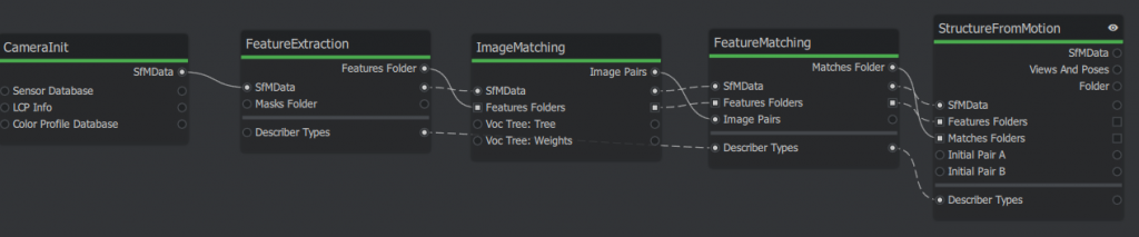
The corresponding script are attached below. Copy and save it as a .mg file then open it as a project in the meshroom GUI. First time running, it may pop upgrade nodes, just agree. There are may dynamic placeholder will be automatically hashed, e.g., {cache}/{nodeType}/{uid0}.
A trick is to clear pending status (in the “⋮” in graphic editor header) and remove all images before passing to Gemini. Because the image info takes a lot of lines.
Source code
{
    "header": {
        "pipelineVersion": "2.2",
        "releaseVersion": "2023.3.0",
        "fileVersion": "1.1",
        "template": false,
        "nodesVersions": {
            "CameraInit": "9.0",
            "StructureFromMotion": "3.3",
            "FeatureExtraction": "1.3",
            "ImageMatching": "2.0",
            "FeatureMatching": "2.0"
        }
    },
    "graph": {
        "CameraInit_1": {
            "nodeType": "CameraInit",
            "position": [0, 0],
            "parallelization": { "blockSize": 0, "size": 0, "split": 1 },
            "uids": { "0": "961e54591174ec5a2457c66da8eadc0cb03d89ba" },
            "internalFolder": "{cache}/{nodeType}/{uid0}/",
            "inputs": {
                "viewpoints": [],
                "intrinsics": [],
                "sensorDatabase": "${ALICEVISION_SENSOR_DB}",
                "defaultFieldOfView": 45.0,
                "viewIdMethod": "metadata"
            },
            "outputs": {
                "output": "{cache}/{nodeType}/{uid0}/cameraInit.sfm"
            }
        },
        "FeatureExtraction_1": {
            "nodeType": "FeatureExtraction",
            "position": [200, 0],
            "parallelization": { "blockSize": 40, "size": 0, "split": 0 },
            "uids": { "0": "7e0174439ccb598ec8c32e23cf2a1da4cd6ab00c" },
            "internalFolder": "{cache}/{nodeType}/{uid0}/",
            "inputs": {
                "input": "{CameraInit_1.output}",
                "describerTypes": ["dspsift"],
                "describerPreset": "normal",
                "describerQuality": "low",
                "forceCpuExtraction": true
            },
            "outputs": {
                "output": "{cache}/{nodeType}/{uid0}/"
            }
        },
        "ImageMatching_1": {
            "nodeType": "ImageMatching",
            "position": [400, 0],
            "parallelization": { "blockSize": 0, "size": 0, "split": 1 },
            "uids": { "0": "896a53c0e4aaf5e02ec421857f1f30439cfe3950" },
            "internalFolder": "{cache}/{nodeType}/{uid0}/",
            "inputs": {
                "input": "{CameraInit_1.output}",
                "featuresFolders": ["{FeatureExtraction_1.output}"],
                "method": "VocabularyTree",
                "tree": "${ALICEVISION_VOCTREE}"
            },
            "outputs": {
                "output": "{cache}/{nodeType}/{uid0}/imageMatches.txt"
            }
        },
        "FeatureMatching_1": {
            "nodeType": "FeatureMatching",
            "position": [600, 0],
            "parallelization": { "blockSize": 20, "size": 0, "split": 0 },
            "uids": { "0": "b446f57fb541abb70e8dc68c47a37e87ec84beff" },
            "internalFolder": "{cache}/{nodeType}/{uid0}/",
            "inputs": {
                "input": "{ImageMatching_1.input}",
                "featuresFolders": "{ImageMatching_1.featuresFolders}",
                "imagePairsList": "{ImageMatching_1.output}",
                "describerTypes": "{FeatureExtraction_1.describerTypes}"
            },
            "outputs": {
                "output": "{cache}/{nodeType}/{uid0}/"
            }
        },
        "StructureFromMotion_1": {
            "nodeType": "StructureFromMotion",
            "position": [800, 0],
            "parallelization": { "blockSize": 0, "size": 0, "split": 1 },
            "uids": { "0": "1d7db1354dab04f156d46106b0b6e27aa0570be3" },
            "internalFolder": "{cache}/{nodeType}/{uid0}/",
            "inputs": {
                "input": "{FeatureMatching_1.input}",
                "featuresFolders": "{FeatureMatching_1.featuresFolders}",
                "matchesFolders": ["{FeatureMatching_1.output}"],
                "describerTypes": "{FeatureMatching_1.describerTypes}",
                "computeStructureColor": true
            },
            "outputs": {
                "output": "{cache}/{nodeType}/{uid0}/sfm.abc"
            }
        }
    }
}Code language: JSON / JSON with Comments (json)
Click Start on top of the panel. The nodes will show different colors: Green – Done; Yellow – Running; Blue – Queueing; Red – Error.
After the SfM node is done, find the reconstructed point cloud in {project-file-dir}/MeshroomCache/StructureFromMotion/{latest-UID}/sfm.abc
The .abc file is efficient for visual effect (VFX) but hard to visualize, so convert it to .ply file using the built-in converter.
# add it to env path in powershell if not yet
$env:ALICEVISION_ROOT = "D:/AYX/Softwares/Meshroom/aliceVision"

## convert .abc to ply
.\aliceVision_exportColoredPointCloud.exe --input "{your_path}\sfm.abc" --output "{your_path}\{file_name}.ply"Code language: PHP (php)
I use python pyvista to visualize them, the colors of the dots are saved under the ‘RGB’ entry.
Python Source Code
import pyvista as pv
import numpy as np
pv.set_jupyter_backend('html')
# Load the PLY you exported
cloud = pv.read(r"{your_file}.ply")
# CRITICAL: Re-center the data to (0,0,0) so you can see it
# We subtract the average position of all points
center = np.mean(cloud.points, axis=0)
cloud.points = cloud.points - center
print(f"Data centered by subtracting: {center}")
# use this to find the color key
print(f'color stored in [{cloud.array_names}]')
# Visualize with PyVista
pl = pv.Plotter()
# Scalars="rgb" ensures the trees and pit look real
pl.add_mesh(cloud, scalars="RGB", rgb=True, point_size=3.0, render_points_as_spheres=True)
pl.add_axes()
pl.show_grid()
pl.show()
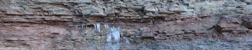
pl.export_html(r'{your_output_path}\preview.html')Code language: PHP (php)Example output show below with an orthophoto for reference. Cameras are colored as green, too. Left Click to orbit, shift + LMouse to pan, Ctrl+LM to pinch rotate, scroll to zoom.
Notes for DJI 3D route planing
fly hub can plan smart 3D scan route but does not support M4T. The slope scan is still valid if we split the cliff into multiple section.
But it needs import 3D reference model.
only obj file available from last scan, try convert it to b3dm. first downsample the obj mesh to 1% of original size for quick test. find a node.js CLI pacakage for {this}. Only do local install for sanity:
npm install {package_folder_name}. After this, run the package from `.\node_module\.bin\{package_executable}`. Turns out this npm is outdated, luckily I installed locally so just remove the node_module and packages.json and package-lock.json from the installed directory everything will be clean.
Another alternative is combining obj2gltf and 3d-tiles-tools, both are CLI tools, but the latter also fails due to complicated C++ dependencies. Thus, only use the obj2gltf.
tried export DTM from google earth Engine Code Editor at https://code.earthengine.google.com/. But it only has 30m
I recall google earth has 3d model, too. Follow this 6 mon ago for video: https://www.youtube.com/watch?v=TUyjF1zgAPo. With a list of software download links:
- Legacy Google Chrome (Portable): https://drive.google.com/file/d/1AGTU…
- RenderDoc 1.31: https://renderdoc.org/stable/1.31/Ren…
- Blender 4.1: https://download.blender.org/release/…
- Maps Models Importer (Blender Addon): https://github.com/eliemichel/MapsMod…
This video {https://www.youtube.com/watch?v=7YRusnTWXjw} is similar but 2 years ago, software may not work anymore. They both follow the same workflow, renderDoc, blender. blender can output as glb, more integrated format. I first join all tiles then export option only select active region, then not more holes.
The pitfall is that the b3dm in fact must follow certain file structure, which is specified from DJI Terra output only. b3dm is actually uses gltf underneath: https://gis.stackexchange.com/questions/272484/what-is-difference-between-b3dm-and-gltf. The b3dm is actually indicate a batch of tiles, easiest way is to use online portal of ceisum ion. upload the `.glb` file the make it availabe for download. I searched many tools for gltf to b3dm conversion but apparently if DJI FH requires DJI terra structure, none of them will work. `py3dtiles` can convert glbf to b3dm, however not sure yet how to adjust the coordinates ( the stackoverflow says the b3dm also uses the glbf underneath)
Ref: https://py3dtiles.org/v5.0.0/api/py3dtiles.tileset.content.b3dm.html
If the 3D route planning won’t work, an alternative is to export flight records saved in `This PC\DJI RC PLUS 2\Internal shared storage\DJI\com.dji.industry.pilot\FlightRecord` and edit them as KMZ. One can read flight record online:
https://www.phantomhelp.com/LogViewer/upload/
Mission summary
Mission overview
Unlike regular task surveying flat objects, the DVPB need to cover vertical cliff surfaces with a low visibility in orthophotos. We first run a regular ortho scan from 80m and upload the photos to a remote server with DJI Terra for quick coarse reconstruction. (DJI Fly Hub2 does not allow free reconstruction online). Then upload the b3dm file from DJI Terra to DJI Fly Hub 2 and overlay it for precise 3D fly route planning. We divide the bowl into 4 tilted surfaces (south, east, north, and a northeast to fill the gap) and carefully adjust the scanned region of each surfaces to avoid collision. All four slope scan routes succeeded as planned. However, it is recommended to manually fly to a position near the starting point of each task then activate the climb to starting point option. Because the auto take-off neglect actual terrain. Similarly, we set exit route mode when the task ends as each task only takes about 5 mins using 10% of battery. It is more efficient to stay and complete all tasks before returning home point.
The slope scan can also be planned on site using AR view. But due to geometry of the bowl, it is hard and risky to get the side view of the scanned surfaces. Therefore, a offline planning is chosen here.
Preference of scanning mode
For global mapping, orthophotos > olibque photos
Less photos are taken but not much resolution lost potentially due to better optimization for ortho scans.
For refined mapping: slope scan > manual scan
The slope scan has more drone motion than the simple view change in manul flight.
Generally: Auto > Manual
Current survey scan route planning is well developed and more advanced than simple manual flight. It is also more tedious to manually to take photos repetitively, a alternative may be time-interval photos to get redundant photos for later reconstruction but overall the automatic routes are more robust and efficient choice on site.
Manual flight
A manual flight is also conducted but the Air Trianglular (point clouds) shows the area with shadow to sun transition has poor coverage. The manul flight is done by tilting cameras vertically with the drone fixed at the center of the bowl. This static drone position may also increase reconstruction difficulty.
Optimize .GLB model size
Reduce glb asset file size:
1) compress png use imagick:
install:
winget install ImageMagick.ImageMagick -e --silent --accept-package-agreements --accept-source-agreements
Use JPEG to compress:
ls *.png | % {
magick "$($_.FullName)" -strip -sampling-factor 4:2:0 -quality 30 "$($_.Directory)\$($_.BaseName).jpg"
}
Then replace all .png to .jpg in the gltf file (essentially a json)
The process can fully automated with https://gltf-transform.dev/
But the compatibility is pretty bad, neither PPT or online viewer can parse it.
2) Faces
Simplify mesh first, originally 160,984 -> shift+D then Esc duplicate
Select object -> Pressure {Tab} -> A (select All) -> M (Merge by distance) with setting to resonable distance -> Reduce to 8,600 faces.
This does not work for reconstruction models, size almost the same, because they are already using jpeg. The number of surfaces are also not decreasing.
Can first decimate then merge then clean up but generally not much to decrease as I guess these reconstructed models are already very optimized.