Photogrammetry Reconstruction

Meshroom photogrammetry reconstruction

The {stack-exchange} post show a free workflow confirmed by {this post}. Among them, Meshroom and {3DF Zephyr Free} seem promising.

Meshroom uses a graphic programming interface, but the graph is saved as json file, thus we can use Gemini (the basic Free Fast version) to write a minimal reconstruction to get point cloud, i.e., structure from motion, sfm. After some auto-correction, the graphs will be obtained:

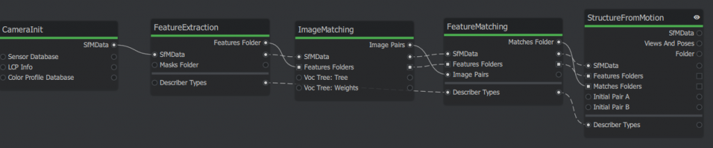
The corresponding script are attached below. Copy and save it as a .mg file then open it as a project in the meshroom GUI. First time running, it may pop upgrade nodes, just agree. There are may dynamic placeholder will be automatically hashed, e.g., {cache}/{nodeType}/{uid0}.
A trick is to clear pending status (in the “⋮” in graphic editor header) and remove all images before passing to Gemini. Because the image info takes a lot of lines.

{
    "header": {
        "pipelineVersion": "2.2",
        "releaseVersion": "2023.3.0",
        "fileVersion": "1.1",
        "template": false,
        "nodesVersions": {
            "CameraInit": "9.0",
            "StructureFromMotion": "3.3",
            "FeatureExtraction": "1.3",
            "ImageMatching": "2.0",
            "FeatureMatching": "2.0"
        }
    },
    "graph": {
        "CameraInit_1": {
            "nodeType": "CameraInit",
            "position": [0, 0],
            "parallelization": { "blockSize": 0, "size": 0, "split": 1 },
            "uids": { "0": "961e54591174ec5a2457c66da8eadc0cb03d89ba" },
            "internalFolder": "{cache}/{nodeType}/{uid0}/",
            "inputs": {
                "viewpoints": [],
                "intrinsics": [],
                "sensorDatabase": "${ALICEVISION_SENSOR_DB}",
                "defaultFieldOfView": 45.0,
                "viewIdMethod": "metadata"
            },
            "outputs": {
                "output": "{cache}/{nodeType}/{uid0}/cameraInit.sfm"
            }
        },
        "FeatureExtraction_1": {
            "nodeType": "FeatureExtraction",
            "position": [200, 0],
            "parallelization": { "blockSize": 40, "size": 0, "split": 0 },
            "uids": { "0": "7e0174439ccb598ec8c32e23cf2a1da4cd6ab00c" },
            "internalFolder": "{cache}/{nodeType}/{uid0}/",
            "inputs": {
                "input": "{CameraInit_1.output}",
                "describerTypes": ["dspsift"],
                "describerPreset": "normal",
                "describerQuality": "low",
                "forceCpuExtraction": true
            },
            "outputs": {
                "output": "{cache}/{nodeType}/{uid0}/"
            }
        },
        "ImageMatching_1": {
            "nodeType": "ImageMatching",
            "position": [400, 0],
            "parallelization": { "blockSize": 0, "size": 0, "split": 1 },
            "uids": { "0": "896a53c0e4aaf5e02ec421857f1f30439cfe3950" },
            "internalFolder": "{cache}/{nodeType}/{uid0}/",
            "inputs": {
                "input": "{CameraInit_1.output}",
                "featuresFolders": ["{FeatureExtraction_1.output}"],
                "method": "VocabularyTree",
                "tree": "${ALICEVISION_VOCTREE}"
            },
            "outputs": {
                "output": "{cache}/{nodeType}/{uid0}/imageMatches.txt"
            }
        },
        "FeatureMatching_1": {
            "nodeType": "FeatureMatching",
            "position": [600, 0],
            "parallelization": { "blockSize": 20, "size": 0, "split": 0 },
            "uids": { "0": "b446f57fb541abb70e8dc68c47a37e87ec84beff" },
            "internalFolder": "{cache}/{nodeType}/{uid0}/",
            "inputs": {
                "input": "{ImageMatching_1.input}",
                "featuresFolders": "{ImageMatching_1.featuresFolders}",
                "imagePairsList": "{ImageMatching_1.output}",
                "describerTypes": "{FeatureExtraction_1.describerTypes}"
            },
            "outputs": {
                "output": "{cache}/{nodeType}/{uid0}/"
            }
        },
        "StructureFromMotion_1": {
            "nodeType": "StructureFromMotion",
            "position": [800, 0],
            "parallelization": { "blockSize": 0, "size": 0, "split": 1 },
            "uids": { "0": "1d7db1354dab04f156d46106b0b6e27aa0570be3" },
            "internalFolder": "{cache}/{nodeType}/{uid0}/",
            "inputs": {
                "input": "{FeatureMatching_1.input}",
                "featuresFolders": "{FeatureMatching_1.featuresFolders}",
                "matchesFolders": ["{FeatureMatching_1.output}"],
                "describerTypes": "{FeatureMatching_1.describerTypes}",
                "computeStructureColor": true
            },
            "outputs": {
                "output": "{cache}/{nodeType}/{uid0}/sfm.abc"
            }
        }
    }
}Code language: JSON / JSON with Comments (json)

Click Start on top of the panel. The nodes will show different colors: Green – Done; Yellow – Running; Blue – Queueing; Red – Error.
After the SfM node is done, find the reconstructed point cloud in {project-file-dir}/MeshroomCache/StructureFromMotion/{latest-UID}/sfm.abc
The .abc file is efficient for visual effect (VFX) but hard to visualize, so convert it to .ply file using the built-in converter.

# add it to env path in powershell if not yet
$env:ALICEVISION_ROOT = "D:/AYX/Softwares/Meshroom/aliceVision"

## convert .abc to ply
.\aliceVision_exportColoredPointCloud.exe --input "{your_path}\sfm.abc" --output "{your_path}\{file_name}.ply"Code language: PHP (php)

I use python pyvista to visualize them, the colors of the dots are saved under the ‘RGB’ entry.

import pyvista as pv
import numpy as np
pv.set_jupyter_backend('html')
# Load the PLY you exported
cloud = pv.read(r"{your_file}.ply")

# CRITICAL: Re-center the data to (0,0,0) so you can see it
# We subtract the average position of all points
center = np.mean(cloud.points, axis=0)
cloud.points = cloud.points - center

print(f"Data centered by subtracting: {center}")

# use this to find the color key
print(f'color stored in [{cloud.array_names}]')

# Visualize with PyVista
pl = pv.Plotter()
# Scalars="rgb" ensures the trees and pit look real
pl.add_mesh(cloud, scalars="RGB", rgb=True, point_size=3.0, render_points_as_spheres=True)
pl.add_axes()
pl.show_grid()
pl.show()
pl.export_html(r'{your_output_path}\preview.html')Code language: PHP (php)

Example output show below with an orthophoto for reference. Cameras are colored as green, too. Left Click to orbit, shift + LMouse to pan, Ctrl+LM to pinch rotate, scroll to zoom.

Notes for DJI 3D route planing

fly hub can plan smart 3D scan route but does not support M4T. The slope scan is still valid if we split the cliff into multiple section.
But it needs import 3D reference model.

only obj file available from last scan, try convert it to b3dm. first downsample the obj mesh to 1% of original size for quick test. find a node.js CLI pacakage for {this}. Only do local install for sanity:
npm install {package_folder_name}. After this, run the package from `.\node_module\.bin\{package_executable}`. Turns out this npm is outdated, luckily I installed locally so just remove the node_module and packages.json and package-lock.json from the installed directory everything will be clean.

Another alternative is combining obj2gltf and 3d-tiles-tools, both are CLI tools, but the latter also fails due to complicated C++ dependencies. Thus, only use the obj2gltf.

tried export DTM from google earth Engine Code Editor at https://code.earthengine.google.com/. But it only has 30m

I recall google earth has 3d model, too. Follow this 6 mon ago for video: https://www.youtube.com/watch?v=TUyjF1zgAPo. With a list of software download links:

• Legacy Google Chrome (Portable): https://drive.google.com/file/d/1AGTU…
• RenderDoc 1.31: https://renderdoc.org/stable/1.31/Ren…
• Blender 4.1: https://download.blender.org/release/…
• Maps Models Importer (Blender Addon): https://github.com/eliemichel/MapsMod…

This video {https://www.youtube.com/watch?v=7YRusnTWXjw} is similar but 2 years ago, software may not work anymore. They both follow the same workflow, renderDoc, blender. blender can output as glb, more integrated format. I first join all tiles then export option only select active region, then not more holes.

The pitfall is that the b3dm in fact must follow certain file structure, which is specified from DJI Terra output only. b3dm is actually uses gltf underneath: https://gis.stackexchange.com/questions/272484/what-is-difference-between-b3dm-and-gltf. The b3dm is actually indicate a batch of tiles, easiest way is to use online portal of ceisum ion. upload the `.glb` file the make it availabe for download. I searched many tools for gltf to b3dm conversion but apparently if DJI FH requires DJI terra structure, none of them will work. `py3dtiles` can convert glbf to b3dm, however not sure yet how to adjust the coordinates ( the stackoverflow says the b3dm also uses the glbf underneath)
Ref: https://py3dtiles.org/v5.0.0/api/py3dtiles.tileset.content.b3dm.html

If the 3D route planning won’t work, an alternative is to export flight records saved in `This PC\DJI RC PLUS 2\Internal shared storage\DJI\com.dji.industry.pilot\FlightRecord` and edit them as KMZ. One can read flight record online:
https://www.phantomhelp.com/LogViewer/upload/

Mission summary

Mission overview

Unlike regular task surveying flat objects, the DVPB need to cover vertical cliff surfaces with a low visibility in orthophotos. We first run a regular ortho scan from 80m and upload the photos to a remote server with DJI Terra for quick coarse reconstruction. (DJI Fly Hub2 does not allow free reconstruction online). Then upload the b3dm file from DJI Terra to DJI Fly Hub 2 and overlay it for precise 3D fly route planning. We divide the bowl into 4 tilted surfaces (south, east, north, and a northeast to fill the gap) and carefully adjust the scanned region of each surfaces to avoid collision. All four slope scan routes succeeded as planned. However, it is recommended to manually fly to a position near the starting point of each task then activate the climb to starting point option. Because the auto take-off neglect actual terrain. Similarly, we set exit route mode when the task ends as each task only takes about 5 mins using 10% of battery. It is more efficient to stay and complete all tasks before returning home point.

The slope scan can also be planned on site using AR view. But due to geometry of the bowl, it is hard and risky to get the side view of the scanned surfaces. Therefore, a offline planning is chosen here.

Preference of scanning mode

For global mapping, orthophotos > olibque photos
Less photos are taken but not much resolution lost potentially due to better optimization for ortho scans.
For refined mapping: slope scan > manual scan
The slope scan has more drone motion than the simple view change in manul flight.
Generally: Auto > Manual
Current survey scan route planning is well developed and more advanced than simple manual flight. It is also more tedious to manually to take photos repetitively, a alternative may be time-interval photos to get redundant photos for later reconstruction but overall the automatic routes are more robust and efficient choice on site.

Manual flight

A manual flight is also conducted but the Air Trianglular (point clouds) shows the area with shadow to sun transition has poor coverage. The manul flight is done by tilting cameras vertically with the drone fixed at the center of the bowl. This static drone position may also increase reconstruction difficulty.